Tokens and Embeddings: The Hidden Language of LLMs

Understanding How Text is Processed and Represented in Transformer-Based LLM Models

If you’re exploring how Large Language Models (LLMs) from OpenAI, Anthropic, or Google work, you’ve likely come across tokenization and embeddings. These foundational concepts transform raw text into a format that LLMs can process and understand, enabling their remarkable language capabilities.

Tokenization and embeddings cover a broad spectrum of techniques. Tokenization breaks text into smaller units, such as subwords, words, or characters, enabling models to process language efficiently. Embeddings, on the other hand, convert these tokens into numerical representations that capture meaning. While classical embeddings like Word2Vec and GloVe provide static word representations, modern transformer-based models generate contextual embeddings that adapt based on surrounding words.

Embeddings have applications beyond text generation, playing a crucial role in tasks like search, sentiment analysis, and text classification—especially in encoder-only models like BERT. However, our focus here is on transformer-based LLMs, which are decoder-only models, and how they utilize tokenization and embeddings to process and generate language.

To keep things clear, we’ll specifically explore how LLMs apply these concepts—focusing on Byte Pair Encoding (BPE) for tokenization and learned embeddings with positional encodings. This way, you’ll gain a solid understanding of how LLMs handle text without getting lost in the broader landscape. Let’s dive in!

Tokenization: Breaking Text into Bite-Sized Pieces

Tokenization is where it all begins. It’s the process of chopping up text into smaller units—called tokens—that the model can chew on. Think of it like cutting a big sandwich into manageable bites. Without tokenization, LLMs wouldn’t know where to start with a sentence like “The cat sat on a mat”. It’s a critical first step because it turns messy, human-written text into a format the model can process. And check out below diagram to see how it works:

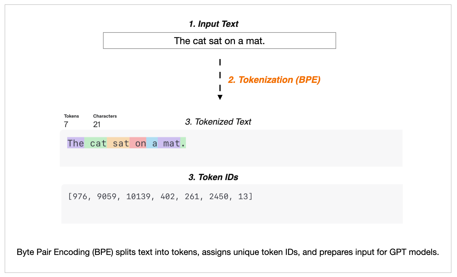
This diagram will illustrate the tokenization pipeline used by OpenAI’s models, showing the progression from raw Input Text through the Byte Pair Encoding (BPE) process to Token IDs, highlighting how common character sequences are transformed into numerical representations for the model.

This diagram will illustrate the tokenization pipeline used by OpenAI’s models, showing the progression from raw Input Text through the Byte Pair Encoding (BPE) process to Token IDs, highlighting how common character sequences are transformed into numerical representations for the model.

As you can see, the process starts with Input Text (or user message), moves to Tokenization (BPE), and ends with Token IDs. Let’s break this down with some technical depth to really understand what’s happening.

Step-by-Step Tokenization with Byte Pair Encoding (BPE)

The diagram will highlight that OpenAI’s models, like those in the GPT family, rely on Byte Pair Encoding (BPE) to tokenize text. BPE, originally a data compression technique, was adapted for NLP and is a game-changer for LLMs. Here’s how it unfolds:

1. Input Text: The raw text—say, “The cat sat on a mat.”—is the starting point. This is just a sequence of characters the model can’t yet use.

2. Tokenization (BPE): BPE splits this text into tokens by identifying and merging the most frequent sequences of characters. The process is iterative:

   • Initialization: Break words into individual characters or byte-level units. For example, “cat” starts as [c, a, t].

   • Frequency Analysis: The algorithm scans a large training corpus to identify the most frequently occurring adjacent pairs of characters or subwords.

   • Merging: The most frequent pair is merged into a single token. For instance, if “ca” frequently appears in the dataset, it may be merged into [ca, t], and later into [cat].

   • Vocabulary Growth: This process continues iteratively until a predefined vocabulary size is reached (e.g., 50,000 tokens in GPT-2), ensuring an efficient balance between token granularity and model performance.

   After BPE processing, each token is assigned a unique token ID—a numerical representation the model can process.

   An example from the diagram will show a sequence like [976, 9059, 10139, 402, 261, 2450, 13]. These are token IDs, unique numerical representations assigned to each token after BPE processing.

3. Token IDs: Once tokens are formed, they’re mapped to unique IDs (e.g., 976 for a token like “The”). These token IDs are what the model uses as input, feeding directly into the embedding layer, where they are transformed into high-dimensional vector representations.

Why BPE Works So Well

BPE’s strength lies in its adaptability. It handles rare words by breaking them into subword units—e.g., “unbelievable” might split into “un,” “believ,” and “able”—ensuring the model can process unseen terms. The byte-level variant, used in GPT-2, starts with a base vocabulary of 256 (all possible byte values), avoiding unknown token issues entirely. This efficiency reduces memory usage and speeds up training, which is critical for scaling LLMs to massive datasets.

Technical Nuances

• Normalization and Pre-tokenization: Before BPE kicks in, text is often normalized (e.g., lowercase) and pre-tokenized into words or basic units, setting the stage for subword splitting.

• Merge Rules: BPE learns merge rules based on frequency in the training data. Suppose “sat” is a frequent subword, BPE may split “sat” into [s, at], then later merge it into [sat] as training progresses. These merges are unique to the dataset and shape how words are broken down.

• Vocabulary Size Impact: The final vocabulary size affects model efficiency. A smaller vocabulary might tokenize “mat” into [m, at], while a larger one might retain [mat] as a single token. OpenAI and other LLM designers optimize this to balance accuracy and compute cost.

Embeddings: Giving Tokens Meaning

Once we’ve got our token IDs from the tokenization step, embeddings step in to give them life. Embeddings are vectors—lists of numbers—that represent each token in a way that captures its meaning. Imagine every token getting its own spot in a giant map where similar words, like “dog” and “puppy,” are parked close together. That’s what embeddings do, and it’s why LLMs can “understand” relationships between words. Let’s dive into this process with the help of this awesome diagram:

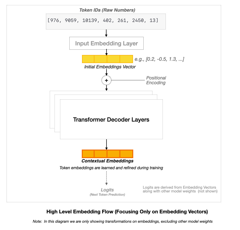
This diagram depict the embedding workflow in a Transformer decoder architecture, showing how Token IDs are converted into Initial Embeddings, enhanced with Positional Encoding, refined through Transformer Decoder Layers into Contextual Embeddings, and finally transformed into Logits for next token prediction.

Note: The above diagram focuses solely on the embedding flow within a Transformer decoder-only model (LLM). It illustrates how token IDs are converted into embeddings and refined through the model. To maintain clarity, it does not depict other essential components of LLMs, such as attention mechanisms and full neural network weight transformations, which contribute to the model’s overall architecture.

This diagram will walk us through how embeddings evolve in an LLM, so let’s break it down step by step.

1. Token IDs (Raw Numbers): The process starts with the token IDs output from BPE, like [976, 9059, 10139, 402, 261, 2450, 13]. These are just integers, but they’re the bridge from text to the model.

2. Input Embedding Layer: Each token ID is looked up in an embedding matrix to get an Initial Embeddings Vector. This matrix, initialized randomly, maps each token ID to a dense vector—e.g., [0.2, -0.5, 1.3, …] for a token like “Cat”. The embedding dimension (e.g., 768 in GPT-2, 1280 in GPT-3) refers to the number of numerical values used to represent each token. A higher dimension captures more nuanced relationships between words but increases computational cost, while a lower dimension is more efficient but may lose some complexity.

   During model training, these vectors are adjusted via backpropagation, allowing the model to learn meaningful relationships between words and concepts, refining how it understands and generates text.

3. Positional Encoding: Unlike earlier sequential models like RNNs and LSTMs, which process text token by token in order, Transformers handle entire sequences in parallel. This parallelism speeds up training but removes the natural sense of order that sequential models have. Transformers don’t inherently know the order of tokens, so Positional Encoding is added to embeddings to introduce token sequence information.

   This positional encoding can be either fixed (using sine and cosine functions, as in the original Transformer) or learned during training (as in models like BERT and GPT). For example, in the sentence “The cat sat on the mat,” the embedding for “cat” is modified with a positional encoding that marks it as the second token in the sequence. Without this step, the model would treat “cat sat” the same as “sat cat,” losing crucial syntactic information, since Transformers process tokens in parallel rather than sequentially.

4. Transformer Decoder Layers: Unlike older models that read text word by word in order, Transformers process everything at once, using self-attention to decide which words matter most in a given context. This makes them great at understanding long-range relationships in text.

   In decoder-only models like GPT, token embeddings (now enriched with positional encodings) pass through multiple Transformer Decoder Layers. These layers refine the embeddings, helping the model understand context. For example, the word “bank” will be represented differently in “river bank” versus “bank account”, because the model learns to interpret words based on surrounding text.

5. Logits (Next Token Prediction): Finally, After passing through the Transformer layers, the model needs to decide what comes next. It does this by turning the refined embeddings into a set of scores (logits), representing how likely each word in its vocabulary is to be the next token.

   We are not dealing with explaining the complete generation process here—that is not the intent of this article. The focus is on how token embeddings evolve through the model, and logits represent the final transformation before a word is chosen.

Why Embeddings Matter

• Semantic Encoding: Initial embeddings capture word relationships, ensuring that similar words (e.g., “cat” and “dog”) are mapped to nearby points in vector space.

• Context Awareness: Transformer layers refine embeddings dynamically, meaning the representation of “sat” in “The cat sat on the mat”depends on the surrounding words.

• Dimensionality Trade-Off: Higher-dimensional embeddings (e.g., 1024 in large models) store richer meaning but require more computational resources—an important balancing act in models like GPT.

Putting It All Together

So, how do tokenization and embeddings team up? It’s a relay race:

• Tokenization: The sentence “The cat sat on the mat” is split into token IDs like [976, 9059, 10139, 402, 261, 2450, 13].

• Embeddings: These token IDs are converted into dense numerical vectors, with positional encodings added to preserve word order.

• Transformation & Training: Through multiple Transformer layers, embeddings are refined during training using self-attention and feed-forward networks. This helps the model adjust word relationships dynamically—so “bank” in “river bank” and “bank account” are understood differently.

• Prediction: These enriched embeddings guide the model in selecting the next token, enabling LLMs to generate fluent and meaningful text.

Wrapping Up

Tokenization and embeddings form the foundation of LLMs. Using BPE, tokenization breaks text into tokens and assigns unique IDs. Embeddings then transform these IDs into rich, context-aware vectors. Together, they enable LLMs to process, understand, and “speak” language in a way that feels almost human. Next time you interact with AI, you’ll have a deeper insight into the language it’s truly understanding and generating.